24 Apply NLP Techniques to Real World Data

24.1 Sentiment Analysis

In this example, we’ll use the IMDB movie review dataset for text classification. We’ll use the pre-trained word embeddings with a Keras model for sentiment analysis.

library(text2vec)
library(keras)
library(tidyverse)

#Load the IMDB dataset:
imdb <- dataset_imdb(num_words = 5000)
x_train <- imdb$train$x
y_train <- imdb$train$y
x_test <- imdb$test$x
y_test <- imdb$test$y

# word_index is a named list mapping words to an integer index
word_index <- dataset_imdb_word_index()

# Reverses it, mapping integer indices to words
reverse_word_index <- names(word_index)                                    
names(reverse_word_index) <- word_index

# Decodes the 1st review. Note that the indices are offset by 3 because 0, 1, and 2 are reserved indices for "padding," "start of sequence," and "unknown."
decoded_review <- sapply(x_train[[1]], function(index) {                
  word <- if (index >= 3) reverse_word_index[[as.character(index - 3)]]
  if (!is.null(word)) word else "?"
})

paste(decoded_review, collapse = " ")

An example of decoded review:

'? this film was just brilliant casting location scenery story direction everyone\'s really suited the part they played and you could just imagine being there robert ? is an amazing actor and now the same being director ? father came from the same scottish island as myself so i loved the fact there was a real connection with this film the witty remarks throughout the film were great it was just brilliant so much that i bought the film as soon as it was released for ? and would recommend it to everyone to watch and the fly ? was amazing really cried at the end it was so sad and you know what they say if you cry at a film it must have been good and this definitely was also ? to the two little ? that played the ? of norman and paul they were just brilliant children are often left out of the ? list i think because the stars that play them all grown up are such a big ? for the whole film but these children are amazing and should be ? for what they have done don\'t you think the whole story was so lovely because it was true and was someone\'s life after all that was ? with us all'
#> [1] "? this film was just brilliant casting location scenery story direction everyone's really suited the part they played and you could just imagine being there robert ? is an amazing actor and now the same being director ? father came from the same scottish island as myself so i loved the fact there was a real connection with this film the witty remarks throughout the film were great it was just brilliant so much that i bought the film as soon as it was released for ? and would recommend it to everyone to watch and the fly ? was amazing really cried at the end it was so sad and you know what they say if you cry at a film it must have been good and this definitely was also ? to the two little ? that played the ? of norman and paul they were just brilliant children are often left out of the ? list i think because the stars that play them all grown up are such a big ? for the whole film but these children are amazing and should be ? for what they have done don't you think the whole story was so lovely because it was true and was someone's life after all that was ? with us all"

In order to feed the data into a neural network, we must first convert the lists of integers into an appropriate tensor format. In this case, we’ll transform the training data into a matrix, where each row consists of 1D vectors.

Each row in the matrix has 5,000 columns, which represent all possible words in a review. These words are then one-hot encoded (also known as categorical encoding), where a 0 or 1 is used to indicate if a specific word is present in the review. This process is performed for each of the 25,000 reviews, resulting in a sparse matrix containing 125,000,000 1s and 0s (occupying 1GB of data). The same transformation is also applied to the testing data, which has an identical size.

library(keras)

vectorize_sequences <- function(sequences, dimension = 5000) {
  # Initialize a matrix with all zeroes
  results <- matrix(0, nrow = length(sequences), ncol = dimension)
  # Replace 0 with a 1 for each column of the matrix given in the list
  for (i in 1:length(sequences))
    results[i, sequences[[i]]] <- 1
  results
}

imdb <- dataset_imdb(num_words = 5000)
x_train <- imdb$train$x
y_train <- imdb$train$y
x_test <- imdb$test$x
y_test <- imdb$test$y

x_train <- vectorize_sequences(x_train)
x_test <- vectorize_sequences(x_test)
y_train <- as.numeric(y_train)
y_test <- as.numeric(y_test)

str(x_train[1,])
#>  num [1:5000] 1 1 0 1 1 1 1 1 1 0 ...

24.2 Building the Network

A type of network that performs well on this kind of vector data is a simple stack of fully connected (dense) layers with ReLU activations.

There are two key architecture decisions to be made when designing such a stack of dense layers:

The number of layers to use
The number of hidden units to choose for each layer

Incorporating more hidden units (a higher-dimensional representation space) enables your network to learn more complex representations, but it also increases the computational cost and may lead to learning unwanted patterns (patterns that enhance performance on the training data but not on the test data).

The chosen model has two intermediate dense layers with 16 hidden units each, and a third (sigmoid) layer that outputs the scalar prediction concerning the sentiment of the current review.

library(keras)

model <- keras_model_sequential() %>%
  layer_dense(units = 16, activation = "relu", input_shape = c(5000)) %>%
  layer_dense(units = 16, activation = "relu") %>%
  layer_dense(units = 1, activation = "sigmoid")

model %>% compile(
  optimizer = "rmsprop",
  loss = "binary_crossentropy",
  metrics = c("accuracy")
)

#prepare the validation dataset
val_indices <- 1:5000

x_val <- x_train[val_indices,]
partial_x_train <- x_train[-val_indices,]
y_val <- y_train[val_indices]
partial_y_train <- y_train[-val_indices]

#fit the model
history <- model %>% fit(
  partial_x_train,
  partial_y_train,
  epochs = 20,
  batch_size = 512,
  validation_data = list(x_val, y_val)
)
#> Epoch 1/20
#> 40/40 - 1s - loss: 0.4940 - accuracy: 0.7876 - val_loss: 0.3602 - val_accuracy: 0.8672 - 1s/epoch - 27ms/step
#> Epoch 2/20
#> 40/40 - 0s - loss: 0.3074 - accuracy: 0.8880 - val_loss: 0.3376 - val_accuracy: 0.8620 - 315ms/epoch - 8ms/step
#> Epoch 3/20
#> 40/40 - 0s - loss: 0.2475 - accuracy: 0.9079 - val_loss: 0.3100 - val_accuracy: 0.8758 - 278ms/epoch - 7ms/step
#> Epoch 4/20
#> 40/40 - 0s - loss: 0.2183 - accuracy: 0.9185 - val_loss: 0.2851 - val_accuracy: 0.8848 - 281ms/epoch - 7ms/step
#> Epoch 5/20
#> 40/40 - 0s - loss: 0.1978 - accuracy: 0.9269 - val_loss: 0.2995 - val_accuracy: 0.8842 - 278ms/epoch - 7ms/step
#> Epoch 6/20
#> 40/40 - 0s - loss: 0.1830 - accuracy: 0.9324 - val_loss: 0.3039 - val_accuracy: 0.8790 - 276ms/epoch - 7ms/step
#> Epoch 7/20
#> 40/40 - 0s - loss: 0.1695 - accuracy: 0.9362 - val_loss: 0.5102 - val_accuracy: 0.8122 - 290ms/epoch - 7ms/step
#> Epoch 8/20
#> 40/40 - 0s - loss: 0.1641 - accuracy: 0.9381 - val_loss: 0.3257 - val_accuracy: 0.8726 - 295ms/epoch - 7ms/step
#> Epoch 9/20
#> 40/40 - 0s - loss: 0.1517 - accuracy: 0.9445 - val_loss: 0.3681 - val_accuracy: 0.8624 - 293ms/epoch - 7ms/step
#> Epoch 10/20
#> 40/40 - 0s - loss: 0.1446 - accuracy: 0.9471 - val_loss: 0.3228 - val_accuracy: 0.8816 - 282ms/epoch - 7ms/step
#> Epoch 11/20
#> 40/40 - 0s - loss: 0.1359 - accuracy: 0.9508 - val_loss: 0.3462 - val_accuracy: 0.8756 - 290ms/epoch - 7ms/step
#> Epoch 12/20
#> 40/40 - 0s - loss: 0.1298 - accuracy: 0.9528 - val_loss: 0.3472 - val_accuracy: 0.8802 - 279ms/epoch - 7ms/step
#> Epoch 13/20
#> 40/40 - 0s - loss: 0.1205 - accuracy: 0.9553 - val_loss: 0.3712 - val_accuracy: 0.8750 - 275ms/epoch - 7ms/step
#> Epoch 14/20
#> 40/40 - 0s - loss: 0.1132 - accuracy: 0.9591 - val_loss: 0.3714 - val_accuracy: 0.8768 - 299ms/epoch - 7ms/step
#> Epoch 15/20
#> 40/40 - 0s - loss: 0.1077 - accuracy: 0.9605 - val_loss: 0.4143 - val_accuracy: 0.8672 - 283ms/epoch - 7ms/step
#> Epoch 16/20
#> 40/40 - 0s - loss: 0.0976 - accuracy: 0.9660 - val_loss: 0.4003 - val_accuracy: 0.8718 - 274ms/epoch - 7ms/step
#> Epoch 17/20
#> 40/40 - 0s - loss: 0.0914 - accuracy: 0.9679 - val_loss: 0.4088 - val_accuracy: 0.8738 - 280ms/epoch - 7ms/step
#> Epoch 18/20
#> 40/40 - 0s - loss: 0.0842 - accuracy: 0.9719 - val_loss: 0.4526 - val_accuracy: 0.8622 - 283ms/epoch - 7ms/step
#> Epoch 19/20
#> 40/40 - 0s - loss: 0.0795 - accuracy: 0.9732 - val_loss: 0.4694 - val_accuracy: 0.8668 - 360ms/epoch - 9ms/step
#> Epoch 20/20
#> 40/40 - 0s - loss: 0.0694 - accuracy: 0.9766 - val_loss: 0.4603 - val_accuracy: 0.8662 - 281ms/epoch - 7ms/step
plot(history)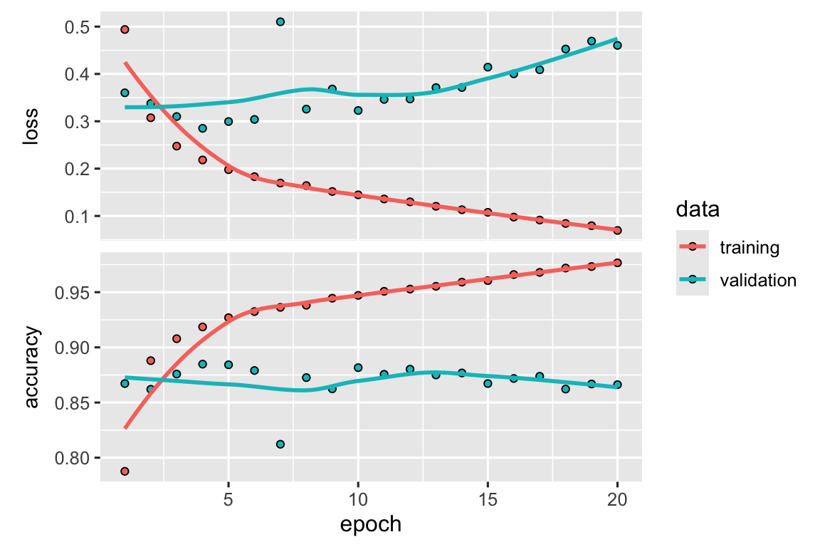

The validation loss and accuracy display signs of overfitting after approximately the 5th epoch, at which point the accuracy reaches its peak and the loss reaches its lowest point. To address this issue, we can limit the training to only 5 epochs.

library(keras)

model <- keras_model_sequential() %>%
  layer_dense(units = 16, activation = "relu", input_shape = c(5000)) %>%
  layer_dense(units = 16, activation = "relu") %>%
  layer_dense(units = 1, activation = "sigmoid")

model %>% compile(
  optimizer = "rmsprop",
  loss = "binary_crossentropy",
  metrics = c("accuracy")
)

model %>% fit(x_train, y_train, epochs = 5, batch_size = 512)
#> Epoch 1/5
#> 49/49 - 1s - loss: 0.4777 - accuracy: 0.7969 - 724ms/epoch - 15ms/step
#> Epoch 2/5
#> 49/49 - 0s - loss: 0.2888 - accuracy: 0.8938 - 276ms/epoch - 6ms/step
#> Epoch 3/5
#> 49/49 - 0s - loss: 0.2380 - accuracy: 0.9107 - 257ms/epoch - 5ms/step
#> Epoch 4/5
#> 49/49 - 0s - loss: 0.2137 - accuracy: 0.9184 - 255ms/epoch - 5ms/step
#> Epoch 5/5
#> 49/49 - 0s - loss: 0.1986 - accuracy: 0.9247 - 286ms/epoch - 6ms/step

results <- model %>% evaluate(x_test, y_test)
#> 782/782 - 1s - loss: 0.3074 - accuracy: 0.8779 - 761ms/epoch - 973us/step
results
#>     loss accuracy 
#> 0.307369 0.877920

Check one review:

library(keras)

#Load the IMDB dataset:
imdb <- dataset_imdb(num_words = 5000)
x_train <- imdb$train$x
y_train <- imdb$train$y
x_test <- imdb$test$x
y_test <- imdb$test$y

# word_index is a named list mapping words to an integer index
word_index <- dataset_imdb_word_index()

# Reverses it, mapping integer indices to words
reverse_word_index <- names(word_index)                                    
names(reverse_word_index) <- word_index

imdb <- dataset_imdb(num_words = 5000)
test_text <- imdb$test$x
decoded_review <- sapply(test_text[[1]], function(index) {                
  word <- if (index >= 3) reverse_word_index[[as.character(index - 3)]]
  if (!is.null(word)) word else "?"
})

paste(decoded_review, collapse = " ")
#> [1] "? please give this one a miss br br ? ? and the rest of the cast ? terrible performances the show is flat flat flat br br i don't know how michael ? could have allowed this one on his ? he almost seemed to know this wasn't going to work out and his performance was quite ? so all you ? fans give this a miss"

The prediction:

  
if (c(model %>% predict(x_test[1:2,]))[1] > 0.5) {
cat('Positive')
} else {
cat('Negative')
}

Output:

print('Negative')
#> [1] "Negative"