5 Data Manipulation Using R
In this section, we will understand how to perform data manipulation using R. We will pay special attention to two of the most used R libraries: dplyr and data.table.
5.1 Overview
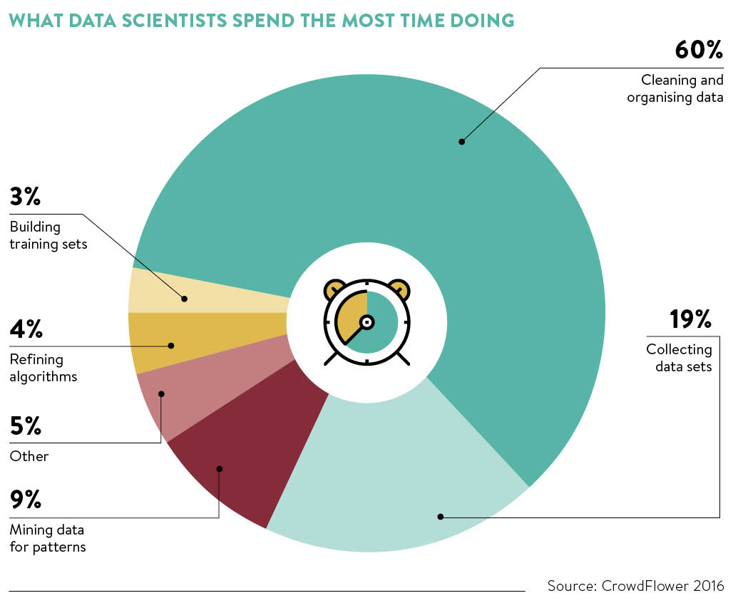
Data manipulation in data science refers to the process of transforming and modifying raw data to make it more suitable for analysis, modeling, and decision-making. It involves various operations such as filtering, sorting, aggregating, joining, reshaping, and creating derived variables. The goal of data manipulation is to organize, clean, and prepare data in a format that facilitates extracting meaningful insights and patterns.
Data manipulation is a critical step in the data science workflow for several reasons:
Data cleaning: Raw data often contains errors, missing values, outliers, or inconsistencies. Data manipulation allows for identifying and addressing these issues through techniques like data validation, imputation, removal of duplicates, and handling missing values. Clean data is essential for accurate analysis and modeling.
Feature engineering: Data manipulation enables the creation of new variables (features) based on existing data, which can capture important patterns and relationships. Feature engineering involves operations such as transforming variables, generating interaction terms, extracting time-based features, and encoding categorical variables. Well-engineered features can significantly enhance the performance of machine learning models.
Data integration: Data manipulation facilitates combining data from multiple sources or tables through operations like merging, joining, or concatenating. This is particularly useful when working with relational databases or when integrating data from different systems. By combining disparate data sources, analysts can gain a comprehensive view and uncover insights that may not be apparent when examining individual datasets.
Data aggregation: Aggregating data involves summarizing or grouping data to derive higher-level insights. Data manipulation allows for aggregating data by factors such as time periods, geographic regions, or customer segments. Aggregating data can provide valuable summary statistics, identify trends, and support decision-making processes.
Data reshaping: Data manipulation allows for transforming data from one format to another, such as pivoting data from a wide format to a long format or vice versa. Reshaping data is useful for various analytical tasks, including data visualization, time series analysis, and data modeling. It enables data to be structured in a way that is most suitable for the analysis at hand.
As a data scientist, you will find most of your time will be spent on exploring your data.
5.2 Data Manipulation with dplyr
The R package dplyr is a powerful and popular package for data manipulation and transformation. It provides a set of functions that offer a consistent and intuitive syntax to perform common data manipulation tasks. dplyr focuses on data frames as the primary data structure and aims to make data manipulation more efficient and user-friendly.
Here’s a brief overview of how to use dplyr:
Creating a data frame: You can create a data frame or load one from external sources (e.g., CSV files) using the
data.frame()function orread.csv()function, respectively.Data manipulation:
dplyrprovides a set of core functions that enable efficient and readable data manipulation. Some commonly used functions include:
- Selecting columns:
select(df, col1, col2) - Filtering rows:
filter(df, condition) - Adding or modifying columns:
mutate(df, new_col = expression) - Arranging rows:
arrange(df, col) - Grouping data:
group_by(df, group_col) - Summarizing data:
summarize(df, new_col = function(col)) - Joining data:
inner_join(df1, df2, by = "key_col")
Piping
%>%operator:dplyrutilizes the%>%operator from the magrittr package, allowing you to chain multiple operations together in a clear and readable manner. This “pipe” operator enhances code readability and reduces the need for intermediate variables.Efficiency and performance:
dplyris designed to be efficient, leveraging optimized C++ code and lazy evaluation. It also integrates well with other packages likedbplyrfor connecting to databases and working with large datasets.
Here is an example:
# Load dplyr package
library(dplyr)
#>
#> Attaching package: 'dplyr'
#> The following objects are masked from 'package:stats':
#>
#>     filter, lag
#> The following objects are masked from 'package:base':
#>
#>     intersect, setdiff, setequal, union

# Create a data frame
df <- data.frame(
  CustomerID = c(1, 1, 2, 2, 3),
  Date = as.Date(c("2023-01-01", "2023-01-05", "2023-01-02", "2023-01-06", "2023-01-03")),
  Product = c("A", "B", "A", "C", "B"),
  Quantity = c(10, 5, 7, 3, 8)
)

# Convert data frame to tibble (optional)
df <- as_tibble(df)

# Subset data and calculate total quantity by product
df_subset <- df %>%
  filter(Date >= as.Date("2023-01-02"), Date <= as.Date("2023-01-05")) %>%
  select(-CustomerID)  # Exclude CustomerID column from output
df_summary <- df_subset %>%
  group_by(Product) %>%
  summarize(TotalQuantity = sum(Quantity))

head(df_summary, 4)
#> # A tibble: 2 × 2
#>   Product TotalQuantity
#>   <chr>           <dbl>
#> 1 A                   7
#> 2 B                  13
5.3 Data Manipulation with data.table
The R package data.table is an efficient and powerful extension of the base R data.frame. It provides a high-performance data manipulation tool with syntax and functionality optimized for large datasets. The primary goal of data.table is to offer fast and memory-efficient operations for handling substantial amounts of data.
Here’s a brief overview of how to use data.table:
Creating a data.table: You can create a data.table from a data.frame or by directly specifying the data.
Data manipulation: data.table provides concise and fast syntax for various data manipulation tasks, including filtering, sorting, aggregating, joining, and updating data. Some commonly used operations include:
- Subset rows using conditions:
dt[condition] - Select columns:
dt[, c("col1", "col2")] - Modify or create columns:
dt[, new_col := expression] - Sort data:
dt[order(col)] - Aggregate
data: dt[, .(mean_col = mean(col)), by = group_col] - Join data:
dt1[dt2, on = "key_col"]
- Efficiency:
data.tableis designed to handle large datasets efficiently. It uses memory-mapped files and optimized algorithms to minimize memory usage and improve performance. Additionally, it provides parallel processing capabilities, allowing you to make use of multiple cores for faster computations.
data.table is especially beneficial in scenarios where you’re working with large datasets and need to perform complex data manipulations quickly. It shines in the following scenarios:
Big data analysis: When dealing with datasets that are too large to fit in memory, data.table provides an efficient solution by minimizing memory usage and optimizing performance.
Speed optimization: data.table is specifically engineered for fast and scalable operations. It outperforms base R and other packages for tasks like subsetting, aggregating, and merging data.
Time-series analysis: data.table offers powerful functionality for working with time-series data, such as rolling joins and efficient grouping and aggregation.
Data cleaning and preprocessing: data.table provides concise and efficient syntax for filtering, transforming, and reshaping data, making it ideal for data cleaning and preprocessing tasks.
Here is an example
# Load data.table package
library(data.table)
#>
#> Attaching package: 'data.table'
#> The following objects are masked from 'package:dplyr':
#>
#>     between, first, last

# Create a data.table
dt <- data.table(
  CustomerID = c(1, 1, 2, 2, 3),
  Date = as.Date(c("2023-01-01", "2023-01-05", "2023-01-02", "2023-01-06", "2023-01-03")),
  Product = c("A", "B", "A", "C", "B"),
  Quantity = c(10, 5, 7, 3, 8)
)

# Subset data and calculate total quantity by product
dt_subset <- dt[Date >= as.Date("2023-01-02") & Date <= as.Date("2023-01-05")]
dt_summary <- dt_subset[, .(TotalQuantity = sum(Quantity)), by = Product]

head(dt_summary, 4)
#>    Product TotalQuantity
#>     <char>         <num>
#> 1:       B            13
#> 2:       A             7
5.4 dplyr vs. data.table
When deciding between data.table and dplyr for data manipulation in R, several factors should be considered. Both packages offer powerful functionality, but they have different design philosophies and performance characteristics. Let’s compare them in terms of syntax, performance, memory usage, functionality, and use cases:
-
Syntax:
-
dplyrhas a more intuitive and expressive syntax that closely resembles natural language. Its function names and the%>%pipe operator contribute to readable and concise code. -
data.tablehas a terser syntax designed for efficiency and speed. It uses square brackets[ ]for subsetting and assignment operations, which can take some time to get used to.
-
-
Performance:
-
data.tableis specifically optimized for fast data manipulation and performs exceptionally well on large datasets. It uses memory-mapped files, efficient indexing, and parallel processing to achieve high performance. -
dplyrperforms well for smaller datasets but may face performance limitations when dealing with very large datasets due to its use of in-memory operations.
-
-
Memory usage:
-
data.tableis memory efficient and optimized for handling large datasets by minimizing memory allocations. It uses a “by-reference” approach, which reduces memory duplication and can be useful for memory-constrained environments. -
dplyris more memory intensive, as it generally creates new copies of data frames during each operation. This can be a disadvantage when working with very large datasets that exceed available memory.
-
-
Functionality:
- Both packages offer similar functionality for data manipulation tasks, including subsetting, filtering, aggregating, and joining data. However, data.table provides additional features like fast grouping, updating columns by reference, and rolling joins, which may not be available or as efficient in
dplyr. -
dplyrhas a broader ecosystem and integrates well with othertidyversepackages, such astidyr andggplot2`, making it convenient for end-to-end data analysis workflows.
- Both packages offer similar functionality for data manipulation tasks, including subsetting, filtering, aggregating, and joining data. However, data.table provides additional features like fast grouping, updating columns by reference, and rolling joins, which may not be available or as efficient in
-
Use cases:
- If you primarily work with large datasets that require efficient and high-performance operations, data.table is a strong choice. It excels in scenarios involving big data, time-series analysis, and situations where speed is crucial.
- If you prioritize code readability, prefer a more intuitive and user-friendly syntax, and work with smaller to medium-sized datasets, dplyr is a good fit. It is well-suited for interactive data exploration, data cleaning, and general data analysis tasks.
It’s worth noting that the choice between data.table and dplyr is not mutually exclusive. Both packages can coexist in the same R environment, allowing you to leverage the strengths of each when appropriate. You can even convert between data.table and dplyr objects using functions like as.data.table() and as_tibble().