library(plotly)
#> Loading required package: ggplot2
#>
#> Attaching package: 'plotly'
#> The following object is masked from 'package:ggplot2':
#>
#>     last_plot
#> The following object is masked from 'package:stats':
#>
#>     filter
#> The following object is masked from 'package:graphics':
#>
#>     layout
library(dendextend)
#>
#> ---------------------
#> Welcome to dendextend version 1.17.1
#> Type citation('dendextend') for how to cite the package.
#>
#> Type browseVignettes(package = 'dendextend') for the package vignette.
#> The github page is: https://github.com/talgalili/dendextend/
#>
#> Suggestions and bug-reports can be submitted at: https://github.com/talgalili/dendextend/issues
#> You may ask questions at stackoverflow, use the r and dendextend tags:
#>   https://stackoverflow.com/questions/tagged/dendextend
#>
#>  To suppress this message use:  suppressPackageStartupMessages(library(dendextend))
#> ---------------------
#>
#> Attaching package: 'dendextend'
#> The following object is masked from 'package:stats':
#>
#>     cutree
library(ggplot2)

# Load iris dataset
data(iris)

# Extract relevant columns for clustering
iris_data <- iris[, 1:4]

# perform hierarchical clustering using complete linkage
dend <- dist(iris_data) %>%
  hclust(method = "complete") %>%
  as.dendrogram()
dend2 <- color_branches(dend, 5)

# plot the dendrogram
p <- ggplot(dend2, horiz = F, offset_labels = -3) + labs(title = "Dendogram")
ggplotly(p)15 Hierarchical Clustering
15.1 Overview
Hierarchical clustering is a type of clustering algorithm used to group similar data points together in a hierarchy. It is an unsupervised learning method, which means that it does not require labeled data. The algorithm creates a hierarchical structure of clusters, with data points that are similar to each other being grouped together.
The two main types of hierarchical clustering are agglomerative and divisive. Agglomerative clustering is more commonly used and works by starting with each data point as a separate cluster and gradually merging them into larger clusters. Divisive clustering, on the other hand, starts with all data points in one cluster and then recursively splits them into smaller clusters.
In agglomerative clustering, the algorithm starts by calculating the distance between each pair of data points and then merges the two closest points into a single cluster. The algorithm then repeats this process, calculating the distance between the new cluster and each of the remaining data points, and merging the closest point or cluster until all data points are part of a single cluster. The resulting hierarchical structure can be represented as a dendrogram, which shows the hierarchical relationships between clusters.
15.2 Implementation of hierarchical clustering
The distance between clusters is typically calculated using a linkage method, which determines how the distance between clusters is measured. The most common linkage methods are: - Single linkage: the distance between the closest pair of data points in the two clusters. - Complete linkage: the distance between the farthest pair of data points in the two clusters. - Average linkage: the average distance between all pairs of data points in the two clusters.
The choice of linkage method can affect the resulting clusters, so it is important to choose an appropriate method based on the characteristics of the data set.
Let’s use the iris dataset to apply the hierarchical clustering:
After performing hierarchical clustering on the data, we can use the resulting dendrogram to determine the appropriate number of clusters. This can be done by specifying a cutoff height at which the dendrogram should be cut to produce the desired number of clusters.
For example, let’s say we have performed hierarchical clustering on a test dataset and obtained a dendrogram. We can visually inspect the dendrogram and determine a cutoff height that results in the desired number of clusters. In this case, let’s say we decide to cut the dendrogram at a distance around 3.4, which would produce 3 clusters.
To implement this in R, we can use the cutree() function to cut the dendrogram at the desired height and obtain the cluster assignments. Here’s an example code:
p <- ggplot(dend2, horiz = F, offset_labels = -3) + geom_hline(aes(yintercept = 3.4, colour = "red")) + labs(title = "Dendogram")
ggplotly(p)
Note that the appropriate cutoff height for the dendrogram may depend on the specific data set and clustering objective, and may require some trial and error to determine.
Let’s also compare it with the K-means algorithm:
library(plotly)
library(cowplot)
library(ggplot2)

km <- kmeans(iris[, 1:4], centers = 3, nstart = 10)
hcl <- hclust(dist(iris[, 1:4]))

df1 = data.frame(PetalLength = iris$Petal.Length, SetalLength=iris$Sepal.Length, cluster = as.factor(km$cluster))

df2 = data.frame(PetalLength = iris$Petal.Length, SetalLength=iris$Sepal.Length, cluster = as.factor(cutree(hcl, k = 3)))

# plots
p1 <- ggplot(df1) +
  aes(x = PetalLength, y = SetalLength, colour = cluster) +
  geom_point(shape = "circle", size = 2) +
  scale_color_hue(direction = 1) +
  labs(title = "K-Means") +
  theme_minimal() +
  theme(plot.title = element_text(size = 10L, face = "bold.italic"))

p2 <- ggplot(df2) +
  aes(x = PetalLength, y = SetalLength, colour = cluster) +
  geom_point(shape = "circle", size = 2) +
  scale_color_hue(direction = 1) +
  labs(title = "Hierarchical Clustering") +
  theme_minimal() +
  theme(plot.title = element_text(size = 10L, face = "bold.italic"))

plot_grid(p1, p2, ncol = 2)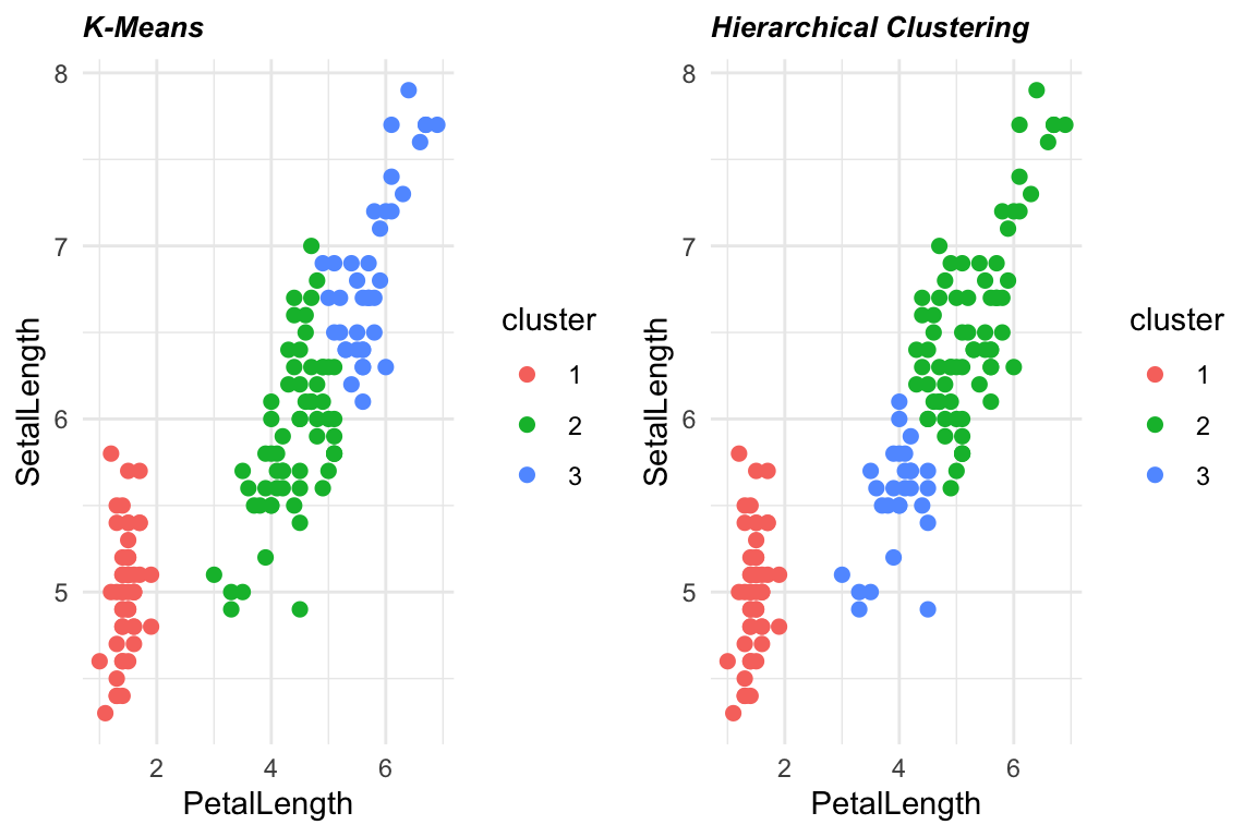
Hierarchical clustering has a number of advantages, such as the ability to create a detailed hierarchical structure of clusters and the absence of the need to specify the number of clusters in advance. However, it can be computationally expensive for large data sets, and the resulting hierarchy can be difficult to interpret for complex data sets.