A widely used nonparametric supervised learning algorithm for classification and regression tasks is the Support Vector Machine (SVM). Introduced in the 1990s by Vapnik and colleagues, SVM aims to find a hyperplane that best separates the input data into different classes.
SVM has several advantages over other classification algorithms. It can handle high-dimensional data well, is less prone to overfitting, and can handle nonlinear data using the kernel trick. Overall, SVM is a powerful and flexible machine learning algorithm applicable in various fields, such as text classification, image classification, and bioinformatics.
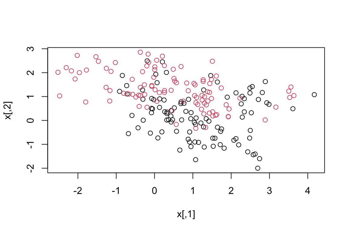
To illustrate the fundamentals of Support Vector Machines (SVM), we can use a straightforward example in R (“ESL.mixture.rda” from the textbook Elements of Statistical Learning). Suppose we have two categories, “red” and “black,” and our dataset has two attributes, “x” and “y.” We aim to construct a classifier that, given a set of (x,y) coordinates, can predict if it belongs to the “red” or “black” category. We can plot our labeled training data on a plane using the following R code:
load(file ="data/ESL.mixture.rda")names(ESL.mixture)#> [1] "x" "y" "xnew" "prob" "marginal" "px1" #> [7] "px2" "means"rm(x, y)#> Warning in rm(x, y): object 'x' not found#> Warning in rm(x, y): object 'y' not foundattach(ESL.mixture)plot(x, col =y+1)
We aim to find a decision boundary that separates these two categories as accurately as possible. This boundary is called the hyperplane in SVM and can be a linear or nonlinear function of the attributes “x” and “y.”
To draw a sample decision boundary in the above code, we can use the svm function from the e1071 package in R. Here is an example code that fits an SVM model with a linear boundary:
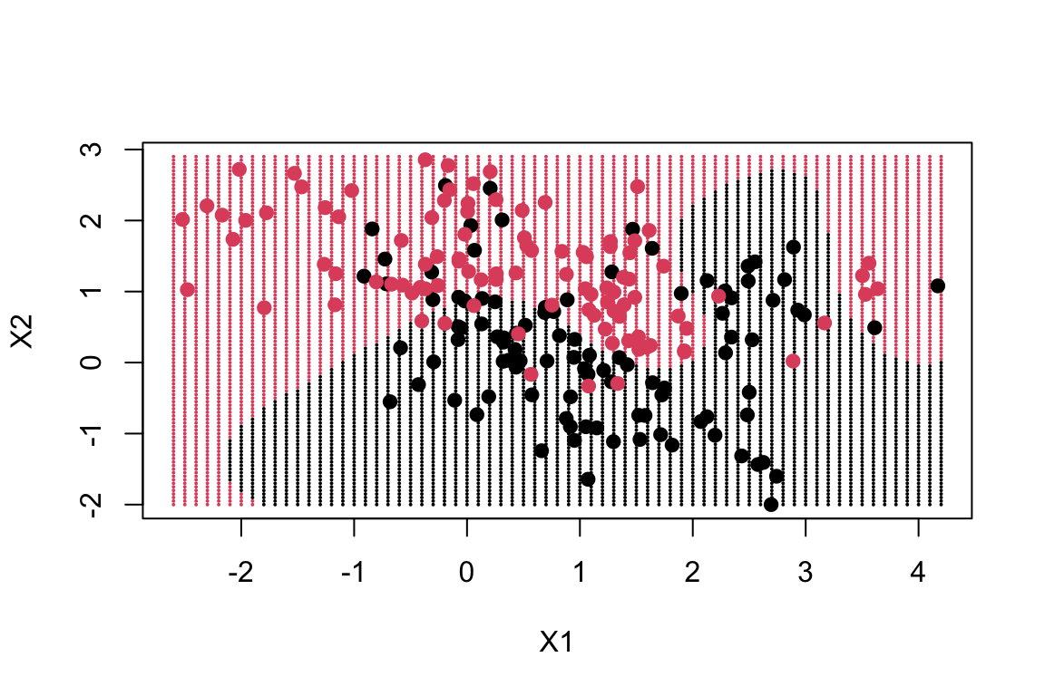
library(e1071)# Fit an SVM model with a linear kerneldat=data.frame(y =factor(y), x)fit=svm(factor(y)~., data =dat, scale =FALSE, kernel ="radial", cost =5)# Make the plotxgrid=expand.grid(X1 =px1, X2 =px2)ygrid=predict(fit, xgrid)plot(xgrid, col =as.numeric(ygrid), pch =20, cex =.2)points(x, col =y+1, pch =19)
The SVM model aims to maximise the margin between the decision boundary and the closest training points from each category (i.e., support vectors). The kernel used in this example allows for a linear decision boundary.
Now let’s move on to the non-linear version of SVM. You’re going to use the kernel support vector machine to try and learn that boundary.
dat=data.frame(y =factor(y), x)fit=svm(factor(y)~., data =dat, scale =FALSE, kernel ="linear", cost =5)fit#> #> Call:#> svm(formula = factor(y) ~ ., data = dat, kernel = "linear", cost = 5, #> scale = FALSE)#> #> #> Parameters:#> SVM-Type: C-classification #> SVM-Kernel: linear #> cost: 5 #> #> Number of Support Vectors: 124
The decision boundary, to a large extent, follows where the data is, but in a very non-linear way.
Support Vector Machines (SVMs) are a type of supervised classifier that can partition a feature space into multiple groups based on known class labels. In simple cases, the separation boundary is linear and leads to groups that are split up by lines or planes in high-dimensional spaces. However, in more complex cases where groups are not nicely separated, SVMs can use a kernel function to carry out non-linear partitioning. This makes them sophisticated and capable classifiers but also prone to overfitting. Despite the black box nature of SVMs, they are useful in situations where the data is non-linearly separated, and their ability to automatically transform data for linear separation makes them a powerful tool. While they may be difficult to interpret, understanding SVMs provides an alternative to GLMs and decision trees for classification.