17 t-Distributed Stochastic Neighbor Embedding
17.1 Overview
t-Distributed Stochastic Neighbour Embedding (t-SNE) is a non-linear dimensionality reduction technique particularly effective for visualising high-dimensional data in a lower-dimensional space. t-SNE is especially useful for data that does not adhere to linear assumptions, where linear techniques like PCA may not provide satisfactory results.
t-SNE operates by attempting to maintain the relative pairwise distances between data points in the high-dimensional space when they are mapped onto a lower-dimensional space. It does so by minimising the divergence between two probability distributions: one representing pairwise similarities in the high-dimensional space, and the other representing pairwise similarities in the lower-dimensional space.
The algorithm involves a stochastic optimisation process, which means that the final results may vary between different runs. Despite this stochastic nature, t-SNE produces visualisations that often reveal the intrinsic structure of the data, such as clusters or groupings.
17.2 The Mathematics of t-SNE
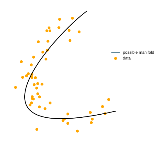
Data in real-life applications can have thousands of dimensions. However, very often, the points lie around a lower-dimensional manifold. In practice, this means that not all features are necessary to represent the data faithfully: by cleverly combining some features, others can be closely approximated.
The problem is, finding this is extremely difficult. There are two main issues. One issue is nonlinearity; the other is the inexact nature of this problem. Putting this into mathematical form, suppose that we have a dataset \[ \mathbf{X} = x_{i=1}^{n}, x_i \in \mathbb{R}^n \] and our goal is to find a lower-dimensional representation \[ \mathbf{Y} = y_{i=1}^{n}, y_i \in \mathbb{R}^m \] where \(n\) is the number of raw features and \(m\) is the number of features after dimensionality reduction (\(m <<< n\)). Popular methods like PCA only work if new features are linear combinations of the old ones. How can this be done for more complex problems? To provide a faithful lower-dimensional representation, we have one main goal in mind: close points should remain tight, distant points shall stay far.
t-SNE achieves this by modeling the dataset with a dimension-agnostic probability distribution, finding a lower-dimensional approximation with a closely matching distribution. It was introduced by Laurens van der Maaten and Geoffrey Hinton in their paper Visualizing High-Dimensional Data Using t-SNE.
Since we also want to capture a possible underlying cluster structure, we define a probability distribution on the \(\mathbf{x}_i\)-s that reflect this. For each data point \(\mathbf{x}_j\), we model the probability of \(\mathbf{x}_i\) belonging to the same class (“being neighbors”) with a Gaussian distribution:

The variance \(\sigma_j\) is a parameter that is essentially given as an input. We don’t set this directly. Instead, we specify the expected number of neighbors, called perplexity.
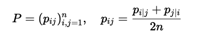
To make the optimization easier, these probabilities are symmetrized. With these symmetric probabilities, we form the distribution \(\mathcal{P}\) that represents our high-dimensional data:
Similarly, we define the distribution \(\mathcal{Q}\) for the \(\mathbf{y}_i\)-s, our (soon to be identified) lower-dimensional representation by
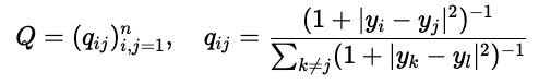
Here, we model the “neighborhood-relation” with the Student t-distribution. This is where the t in t-SNE comes from.
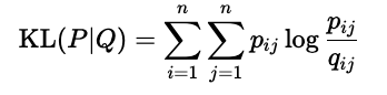
Our goal is to find the \(\mathbf{y}_i\)-s through optimization such that \(\mathcal{P}\) and \(\mathcal{Q}\) are as close together as possible. (In a distributional sense.) This closeness is expressed with the Kullback-Leibler divergence, defined by:
We have successfully formulated the dimensionality reduction problem as optimization!
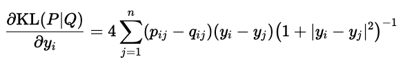
From here, we calculate the gradient of KL divergence with respect to the \(\mathbf{y}_i\)-s and find an optimum with gradient descent. Fortunately, we can calculate the gradient simply:
17.3 An R Example
In R, the Rtsne function from the Rtsne package can be used to perform t-SNE. Before applying t-SNE to the Iris dataset, it’s necessary to remove any duplicated entries. Here’s an example of how to do this:
library(Rtsne)
library(ggplot2)
library(plotly)
#>
#> Attaching package: 'plotly'
#> The following object is masked from 'package:ggplot2':
#>
#>     last_plot
#> The following object is masked from 'package:stats':
#>
#>     filter
#> The following object is masked from 'package:graphics':
#>
#>     layout

# Load the iris dataset
data(iris)

# Remove duplicated entries in the iris dataset
iris_unique <- unique(iris)

# Perform t-SNE on the iris data (excluding the Species column)
tsne_result <- Rtsne(iris_unique[, -5], check_duplicates = FALSE)
df_tsne <- data.frame(tsne_result$Y, Species = as.factor(iris_unique$Species))

p <- ggplot(df_tsne) +
  aes(x = X1, y = X2, colour = Species) +
  geom_point(shape = "circle", size = 2) +
  scale_color_hue(direction = 1) +
  labs(title = "t-SNE Clustering") +
  theme_minimal() +
  theme(plot.title = element_text(size = 10L, face = "bold.italic"))

ggplotly(p)
As with PCA, t-SNE visualisations can help reveal the underlying structure of high-dimensional data, such as clusters, groupings, or other patterns. However, it is essential to consider that the distances between clusters in the lower-dimensional space do not always accurately represent their distances in the high-dimensional space.
Additionally, careful selection of hyper parameters can further enhance the quality of the clustering. t-SNE, along with numerous other methods, particularly classification algorithms, possesses two critical parameters that can greatly impact the clustering of the data:
Perplexity: This parameter balances the global and local aspects of the data. A higher perplexity value emphasises global relationships, while a lower value highlights local relationships. Choosing an appropriate perplexity value is essential for obtaining meaningful visualisations.
Iterations: This parameter specifies the number of iterations before the clustering process is halted. Increasing the number of iterations may lead to a more stable and accurate representation of the data. However, it may also increase the computational time required to perform the analysis.
Despite these limitations, t-SNE provides a powerful tool for visualising high-dimensional data, especially when linear techniques like PCA are not suitable.